
|
|
Boost : |
Subject: Re: [boost] Boost.Plot? - Scalable Vector Graphics (was [expressive] performance tuning
From: Edward Grace (ej.grace_at_[hidden])
Date: 2009-07-31 14:19:43
[ Warning to all - the following is a long, complex response -- don't
bother reading unless you are *really* interested in the pedantic
nuances of timing stuff! It may cause your eyes to glaze over and
loss of consciousness.
Apologies also for clogging up inboxes with pngs - be thankful for
the mailing sentry bouncing this thing out until it got short enough!
It just didn't read well with hyperlinked pictures. ]
On 30 Jul 2009, at 23:21, Simonson, Lucanus J wrote:
> Edward Grace wrote:
>>> Personally I perform several runs of the same benchmark and then
>>> take the minimum time as the time I report.
>>
>> Be very cautious about that for a number of reasons.
>>
>> a) By reporting the minimum, without qualifying your statement, you
>> are lying. For example if you say "My code takes 10.112 seconds to
>> run." people are unlikely to ever observe that time - it is by
>> construction atypical.
>
> I try to be explicit about explaining what metric I'm reporting.
> If I'm reporting the minimum of ten trials I report it as the
> minimum of ten trials.
Good show!
Re-reading my comments, it looks a bit adversarial - it's not
intended to be! I'm not accusing you of falsehood or dodgy dealings!
Apologies if that was the apparent tone!
> Taking the minimum of ten trials and comparing it to the minimum
> of twenty trials and not qaulifying it would be even more dishonest
> because it isn't fair. I compare same number of trails, report
> that it is the minimum and the number of trails.
>
>> b) If ever you do this (use the minimum or maximum) then you are
>> unwittingly sampling an extreme value distribution:
>>
>> http://en.wikipedia.org/wiki/Extreme_value_distribution
>>
>> For example - say you 'know' that the measured times are normally
>> distributed with mean (and median) zero and a variance of 10. If you
[...]
>> scenario. Notice that the histogram of the observed minimum is *far*
>> broader than the observed median.
>
> In this particular case of runtime the distribution is usually not
> normal.
Of course, hence the quotes around 'know'. My demonstration of the
effect of taking the minimum is based on the normal distribution
since everyone knows it and it's assumed to be 'nice'. If you repeat
what I did with another distribution (e.g. uniform, or Pareto) both
of which have a well defined minimum you will still see the same
effect! In fact, you are likely to observe even more extreme
behaviour! I did not discuss more realistic distributions since it
would cause people's eyes to glaze over even faster than this will!
> There is some theoritical fastest the program could go if nothing
> like the OS or execution of other programs on the same machine
> cause it to run slower. This is the number we actually want. We
> can't measure it, but we observe that there is a "floor" under our
> data and the more times we run the more clear it becomes where that
> floor is.
Sure. This is partially a philosophical point regarding what one is
trying to measure. In your case if you are trying to determine the
fastest speed that the code could possibly go (and you don't have a
real-time OS) then the minimum observed time looks like a good idea.
I don't object to the use of the minimum (or any other estimator) per
se, at least not yet. What one wishes to measure should determine
the choice of estimator.
For example, I do not want to know the minimum possible time as that
is not indicative of the typical time. I want to compare the typical
execution times of two codes *with* the OS taken in to account since,
in the real world, this is what a user will notice and therefore what
matters to me.
Paraphrasing "Hamlet",
'To median or not to median - that is not quite the question.'
My point is far more subtle than I think you have appreciated.
The crux is that whatever your estimator you need to understand how
it's distributed if you want to infer anything from it. So, if you
*are* going to use the minimum (which is not robust) then you need to
be aware that you may be inadvertently bitten by extreme value theory
- consequently you should consider the form of the dispersion - it
sure as heck won't be normal! This may seem bizarre - these things
often are!
To give you a concrete example, consider the following code (this
also contains PDFs of the plots):
Here, we crudely time a simple function using a given number of
iterations in a fairly typical manner. We repeat this timing 4001
times and then report the minimum and median of these 4001
acquisitions. This constitutes 'a measurement'.
Each experimental 'measurement' is carried out for a randomly chosen
number of iterations of the main timing loop and is hopefully
independent. This is to try and satisfy the first i in iid
(independent and identically distributed).
For those of you bash oriented I do:
./ejg-make-input-for-empirical-ev > inputs.dat
rm test.dat; while read line; do echo $line; echo $line | ./ejg-
empirical-ev >> test.dat; done < inputs.dat
No attempt is made to 'sanitise' the computer, nor do I deliberately
load it.
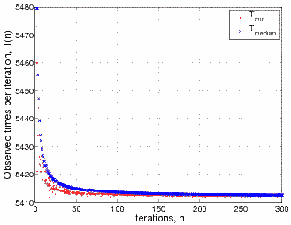
The raw results are shown below,
The most obvious observation is that as the number of iterations
increases the times both appear to converge in an asymptotic-like
manner towards some 'true' value. This is clearly the effect of some
overhead (e.g. the time taken to call the clock) having progressively
less impact on the overall time. Secondly, the minimum observed time
is lower than the median (as expected).
What you may find a little surprising is that the *variation* of the
minimum observed time is far greater than the variation in the median
observed time. This is the key to my warning!
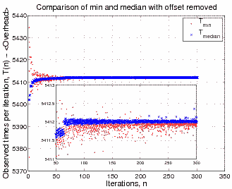
If we crudely account for the overhead of the clock (which of course
will also be stochastic - but let's ignore that) and subtract it then
this phenomenon becomes even more stark.
The variation of the observed times is now far clearer. Also, notice
that rogue-looking red point in the bottom left of the main plot -
for small numbers of iterations the dispersion of the minimum is
massive compared to the dispersion of the median. You will also
notice that there's now little difference between the predominant
value of the median and minimum in this case.
Now consider the inset, the second obvious characteristic is that the
times do not appear to fluctuate entirely randomly with iteration
number - instead there is obvious structure - indeed a sudden jump in
behaviour around n=60. This is likely to be a strong interference
effect between the clock and the function that's being measured and
other architecture dependent issues (e.g. cache) that I won't pretend
to fully understand.
It's also indicative of how to interpret the observed variation -
it's not necessarily purely random, but random + pseudorandom. Like
std::rand(), if you keep the same seed (number of iterations) you may
well observe the same result. That does not however mean that your
true variance is zero - it's just hidden!
Looking at the zoom in the inset it's clear to see that the median
time has a generally far lower dispersion than the minimum time (by
around an order of magnitude). There are even situations where the
minimum time is clearly greater than the median time - directly
counter to your expectation. This is not universally the case, but
the general behaviour is perfectly clear.
This can be considered to be a direct result of extreme value
theory. If you use the minimum (or similar quantile) to estimate
something about a random variable the result may have a large
dispersion (variance) compared to the median. Just because you
haven't seen it (changed the seed in your random number generator)
doesn't mean it's not there!
The practical amongst you may well say "Hey - who cares, we're
talking about tiny differences!"
I agree!
So, is the moral of this tale to avoid using the minimum and instead
to use the median? Not at all. I'm agnostic on this issue for
reasons I mentioned above, however when / if one uses the minimum one
needs to be careful and be aware of the (hidden) assumptions! For
example, as various aspects of the timing change one may observe a
sudden change in the cdf, 'magic' in the cache could perhaps cause
the median measure to change far more than the minimum measure - so
even though median may have better nominal precision, the minimum may
well have better nominal accuracy. If you look in the code you'll
see evidence that I've mucked around with different quantiles - I
have not closed my mind to using the minimum!
> It just won't run faster than that no matter how often we run.
Have you tried varying the number of iterations? You'll find that
for some iteration lengths it may go significantly faster - doubtless
this is a machine architecture issue, I don't know why - but it happens.
> The idea is that using the minimum as the metric eliminates most of
> the "noise" introduced into the data by stuff unrelated to what you
> are trying to measure. Taking the median is just taking the median
> of the noise.
Not necessarily - as you can see from the above plots. Just because
your estimator is repeatable for a given number of iterations doesn't
mean it's 'ok' or eliminated the 'noise' - it's far more subtle than
that.
> In an ideal compute environment your runtimes would be so similar
> from run to run you wouldn't bother to run more than once. If
> there is noise in your data set your statistic should be designed
> to eliminate the noise, not characterize it.
If you want to try and eliminate it you need to characterise it.
This is why relative measurements are so important if you desire
precision - the noise is always there, no matter what you do, so
having 'well behaved' noise (e.g. asymptotically normal) means you
can infer things in a meaningful manner when you take differences.
If you have no idea what the form of your noise is - or think you've
eliminated it you can get repeatable results but they may be a subtle
distortion of the truth. By taking the minimum you are not
necessarily avoiding the 'noise', you may think you are - indeed it
may look like you are, but you could have just done a good job of
hiding it!
> In my recent boostcon presentation my benchmarks were all for a
> single trial of each algorithm for each benchmark because noise
> would be eliminated during the curve fitting of the data for
> analysis of how well the algorithms scaled (if not by the
> conversion to logarithmic axis....)
As an aside you may find least absolute deviation (LAD) regression
more appropriate than ordinary least squares (I'm assuming you used
OLS of course).
For practical application what you've done is almost certainly fine,
'good enough for government work' as the saying goes - I'm not
suggesting it isn't. After all, as I have already commented, when
human experimenters are involved we can eyeball the results and see
when things look fishy or don't behave as expected.
Ultimately - the take away message is apparently axiomatic 'truths'
are not always as true as one might think.
A dark art indeed! ;-)
-ed
------------------------------------------------
"No more boom and bust." -- Dr. J. G. Brown, 1997
Boost list run by bdawes at acm.org, gregod at cs.rpi.edu, cpdaniel at pacbell.net, john at johnmaddock.co.uk